Update Meeting: 29-11-2021
Jenny Sjaarda
2021-11-01
Last updated: 2021-11-29
Checks: 7 0
Knit directory: proxyMR/
This reproducible R Markdown analysis was created with workflowr (version 1.6.2). The Checks tab describes the reproducibility checks that were applied when the results were created. The Past versions tab lists the development history.
Great! Since the R Markdown file has been committed to the Git repository, you know the exact version of the code that produced these results.
Great job! The global environment was empty. Objects defined in the global environment can affect the analysis in your R Markdown file in unknown ways. For reproduciblity it's best to always run the code in an empty environment.
The command set.seed(20210602) was run prior to running the code in the R Markdown file. Setting a seed ensures that any results that rely on randomness, e.g. subsampling or permutations, are reproducible.
Great job! Recording the operating system, R version, and package versions is critical for reproducibility.
Nice! There were no cached chunks for this analysis, so you can be confident that you successfully produced the results during this run.
Great job! Using relative paths to the files within your workflowr project makes it easier to run your code on other machines.
Great! You are using Git for version control. Tracking code development and connecting the code version to the results is critical for reproducibility.
The results in this page were generated with repository version a836698. See the Past versions tab to see a history of the changes made to the R Markdown and HTML files.
Note that you need to be careful to ensure that all relevant files for the analysis have been committed to Git prior to generating the results (you can use wflow_publish or wflow_git_commit). workflowr only checks the R Markdown file, but you know if there are other scripts or data files that it depends on. Below is the status of the Git repository when the results were generated:
Ignored files:
    Ignored:    .Rhistory
    Ignored:    .Rproj.user/
    Ignored:    _targets/
    Ignored:    analysis/_site.yml_cp
    Ignored:    analysis/bgenie_GWAS/
    Ignored:    analysis/data_setup/
    Ignored:    analysis/download_Neale_list.csv
    Ignored:    analysis/process_Neale.out
    Ignored:    analysis/traitMR/
    Ignored:    data/Neale_SGG_directory_12_07_2021.csv
    Ignored:    data/Neale_SGG_directory_15_07_2021.csv
    Ignored:    data/PHESANT_file_directory_05_10_2021.txt
    Ignored:    data/UKBB_pheno_directory_05_10_2021.csv
    Ignored:    data/processed/
    Ignored:    data/raw/
    Ignored:    output/figures/
    Ignored:    output/tables/traitMR/
    Ignored:    proxyMR_comparison.RData
    Ignored:    proxyMR_figure_data.RData
    Ignored:    proxymr_100_clustermq.out
    Ignored:    proxymr_101_clustermq.out
    Ignored:    proxymr_102_clustermq.out
    Ignored:    proxymr_103_clustermq.out
    Ignored:    proxymr_104_clustermq.out
    Ignored:    proxymr_105_clustermq.out
    Ignored:    proxymr_106_clustermq.out
    Ignored:    proxymr_107_clustermq.out
    Ignored:    proxymr_108_clustermq.out
    Ignored:    proxymr_109_clustermq.out
    Ignored:    proxymr_10_clustermq.out
    Ignored:    proxymr_110_clustermq.out
    Ignored:    proxymr_111_clustermq.out
    Ignored:    proxymr_112_clustermq.out
    Ignored:    proxymr_113_clustermq.out
    Ignored:    proxymr_114_clustermq.out
    Ignored:    proxymr_115_clustermq.out
    Ignored:    proxymr_116_clustermq.out
    Ignored:    proxymr_117_clustermq.out
    Ignored:    proxymr_118_clustermq.out
    Ignored:    proxymr_119_clustermq.out
    Ignored:    proxymr_11_clustermq.out
    Ignored:    proxymr_120_clustermq.out
    Ignored:    proxymr_121_clustermq.out
    Ignored:    proxymr_122_clustermq.out
    Ignored:    proxymr_123_clustermq.out
    Ignored:    proxymr_124_clustermq.out
    Ignored:    proxymr_125_clustermq.out
    Ignored:    proxymr_126_clustermq.out
    Ignored:    proxymr_127_clustermq.out
    Ignored:    proxymr_128_clustermq.out
    Ignored:    proxymr_129_clustermq.out
    Ignored:    proxymr_12_clustermq.out
    Ignored:    proxymr_130_clustermq.out
    Ignored:    proxymr_131_clustermq.out
    Ignored:    proxymr_132_clustermq.out
    Ignored:    proxymr_133_clustermq.out
    Ignored:    proxymr_134_clustermq.out
    Ignored:    proxymr_135_clustermq.out
    Ignored:    proxymr_136_clustermq.out
    Ignored:    proxymr_137_clustermq.out
    Ignored:    proxymr_138_clustermq.out
    Ignored:    proxymr_139_clustermq.out
    Ignored:    proxymr_13_clustermq.out
    Ignored:    proxymr_140_clustermq.out
    Ignored:    proxymr_14_clustermq.out
    Ignored:    proxymr_15_clustermq.out
    Ignored:    proxymr_16_clustermq.out
    Ignored:    proxymr_17_clustermq.out
    Ignored:    proxymr_18_clustermq.out
    Ignored:    proxymr_19_clustermq.out
    Ignored:    proxymr_1_clustermq.out
    Ignored:    proxymr_20_clustermq.out
    Ignored:    proxymr_21_clustermq.out
    Ignored:    proxymr_22_clustermq.out
    Ignored:    proxymr_23_clustermq.out
    Ignored:    proxymr_24_clustermq.out
    Ignored:    proxymr_25_clustermq.out
    Ignored:    proxymr_26_clustermq.out
    Ignored:    proxymr_27_clustermq.out
    Ignored:    proxymr_28_clustermq.out
    Ignored:    proxymr_29_clustermq.out
    Ignored:    proxymr_2_clustermq.out
    Ignored:    proxymr_30_clustermq.out
    Ignored:    proxymr_31_clustermq.out
    Ignored:    proxymr_32_clustermq.out
    Ignored:    proxymr_33_clustermq.out
    Ignored:    proxymr_34_clustermq.out
    Ignored:    proxymr_35_clustermq.out
    Ignored:    proxymr_36_clustermq.out
    Ignored:    proxymr_37_clustermq.out
    Ignored:    proxymr_38_clustermq.out
    Ignored:    proxymr_39_clustermq.out
    Ignored:    proxymr_3_clustermq.out
    Ignored:    proxymr_40_clustermq.out
    Ignored:    proxymr_41_clustermq.out
    Ignored:    proxymr_42_clustermq.out
    Ignored:    proxymr_43_clustermq.out
    Ignored:    proxymr_44_clustermq.out
    Ignored:    proxymr_45_clustermq.out
    Ignored:    proxymr_46_clustermq.out
    Ignored:    proxymr_47_clustermq.out
    Ignored:    proxymr_48_clustermq.out
    Ignored:    proxymr_49_clustermq.out
    Ignored:    proxymr_4_clustermq.out
    Ignored:    proxymr_50_clustermq.out
    Ignored:    proxymr_51_clustermq.out
    Ignored:    proxymr_52_clustermq.out
    Ignored:    proxymr_53_clustermq.out
    Ignored:    proxymr_54_clustermq.out
    Ignored:    proxymr_55_clustermq.out
    Ignored:    proxymr_56_clustermq.out
    Ignored:    proxymr_57_clustermq.out
    Ignored:    proxymr_58_clustermq.out
    Ignored:    proxymr_59_clustermq.out
    Ignored:    proxymr_5_clustermq.out
    Ignored:    proxymr_60_clustermq.out
    Ignored:    proxymr_61_clustermq.out
    Ignored:    proxymr_62_clustermq.out
    Ignored:    proxymr_63_clustermq.out
    Ignored:    proxymr_64_clustermq.out
    Ignored:    proxymr_65_clustermq.out
    Ignored:    proxymr_66_clustermq.out
    Ignored:    proxymr_67_clustermq.out
    Ignored:    proxymr_68_clustermq.out
    Ignored:    proxymr_69_clustermq.out
    Ignored:    proxymr_6_clustermq.out
    Ignored:    proxymr_70_clustermq.out
    Ignored:    proxymr_71_clustermq.out
    Ignored:    proxymr_72_clustermq.out
    Ignored:    proxymr_73_clustermq.out
    Ignored:    proxymr_74_clustermq.out
    Ignored:    proxymr_75_clustermq.out
    Ignored:    proxymr_76_clustermq.out
    Ignored:    proxymr_77_clustermq.out
    Ignored:    proxymr_78_clustermq.out
    Ignored:    proxymr_79_clustermq.out
    Ignored:    proxymr_7_clustermq.out
    Ignored:    proxymr_80_clustermq.out
    Ignored:    proxymr_81_clustermq.out
    Ignored:    proxymr_82_clustermq.out
    Ignored:    proxymr_83_clustermq.out
    Ignored:    proxymr_84_clustermq.out
    Ignored:    proxymr_85_clustermq.out
    Ignored:    proxymr_86_clustermq.out
    Ignored:    proxymr_87_clustermq.out
    Ignored:    proxymr_88_clustermq.out
    Ignored:    proxymr_89_clustermq.out
    Ignored:    proxymr_8_clustermq.out
    Ignored:    proxymr_90_clustermq.out
    Ignored:    proxymr_91_clustermq.out
    Ignored:    proxymr_92_clustermq.out
    Ignored:    proxymr_93_clustermq.out
    Ignored:    proxymr_94_clustermq.out
    Ignored:    proxymr_95_clustermq.out
    Ignored:    proxymr_96_clustermq.out
    Ignored:    proxymr_97_clustermq.out
    Ignored:    proxymr_98_clustermq.out
    Ignored:    proxymr_99_clustermq.out
    Ignored:    proxymr_9_clustermq.out
    Ignored:    renv/library/
    Ignored:    renv/staging/

Untracked files:
    Untracked:  Rplots.pdf

Unstaged changes:
    Modified:   analysis/AM_MR_summary.Rmd
    Modified:   output/tables/define_Neale_categories.csv
    Modified:   output/tables/define_Neale_categories_filled.csv
    Modified:   renv.lock
Note that any generated files, e.g. HTML, png, CSS, etc., are not included in this status report because it is ok for generated content to have uncommitted changes.
These are the previous versions of the repository in which changes were made to the R Markdown (analysis/update_meeting_29_11_2021.Rmd) and HTML (docs/update_meeting_29_11_2021.html) files. If you've configured a remote Git repository (see ?wflow_git_remote), click on the hyperlinks in the table below to view the files as they were in that past version.
| File | Version | Author | Date | Message |
|---|---|---|---|---|
| Rmd | a836698 | Jenny Sjaarda | 2021-11-29 | wflow_publish("analysis/update_meeting_29_11_2021.Rmd") |
| Rmd | 3abb0a0 | jennysjaarda | 2021-11-28 | add udpate meeting for 29/11/21 |
1 Analyses update.
1.1 MR effects vs. raw correlation.
Sought to compare the raw correlation amongst couples vs. the standardized MR effects. There are many traits where the correlation > MR effects including some traits of interest such as standing height, place of birth, among many others. A plot comparing the two and a summary table of the effects is shown below.
1.2 Same-trait analyses.
A few key changes to the pipeline since last time we looked at these results:
- List of traits of interest changed to exclude dietary traits and add binary traits (among a few other minor revisions), total number of traits went down.
- Sample changed to ensure both males and females were not related (previously had only removed unrelated within males and females separately), our resulting samples closely matched Neale round 2 GWAS which resulted in much fewer couples (~50K instead of ~65K).
- Filtered SNPs for evidence of reverse causality (should not have any bearing on these results since these involve only one trait).
- Meta-analyses are performed at SNP-level rather than MR-level.
1.2.1 Re-calculate number of significant results in same trait analyses.
- The number of analyses corresponds to the number of traits (110).
- The significant results after adjusting for multiple hypothesis testing are shown below.
IVW_meta_betaandIVW_meta_pvalcorresponds to the beta and p-value of the meta-analyzed MR across sexes, respectively (i.e. MR estimates were computed in each sex-seperately using sex-specific SNP-exposure and SNP-outcome results and then meta-analyzed).- After adjusting for multiple tests (p <
0.05/62), identified 60 significant assortative mating MR results (corresponding to the table below).
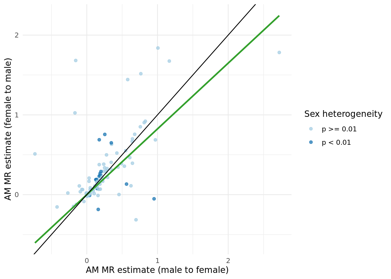
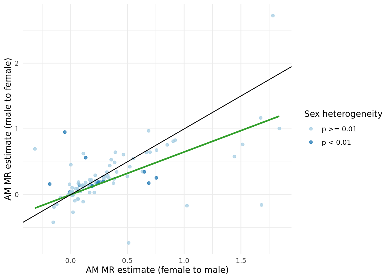
1.2.2 Sex heterogeneity.
- For each AM MR (\(X_{p} \sim X_i\)), analyses were run in each sex separately.
- Of the significant results shown above, we tested to see if there was any difference in AM MR estimates between sexes.
- A similar adjustment for multiple hypothesis testing was applied as above, resulting in 28 number of effective tests.
- After adjusting for multiple hypothesis testing (p <
0.05/28), 0 traits showed significant differences amongst sexes (this changed from before). - The table below shows the nominally significant results at
p < 0.05.
Figures compared the male to female MR results, and vice versa are shown below. Suggests evidence of regression dilution bias?
1.2.3 Binned results.
- For each AM MR (\(X_{p} \sim X_i\)), analyses were run in the full sample as well as in 5 roughly equal sized bins according to time couple had been together (
time_together_even_bins) estimated using time at household variable, and median age (age_even_bins). - Of the 60 significant results shown above, we tested to see if there was any significant difference in AM MR estimates amongst the two grouping variables.
- Specifically, the outcome data set was split into 5 bins, and the SNP-outcome effect was estimated in each bin separately (and each sex seperately).
- These outcome-SNP effects were then used to generate bin-specific MR estimates, using the same SNP-exposure effects from Neale.
- To estimate the difference among bins, we used two approaches:
- The Cochran's Q test to test for heterogeneity in meta-analyses (of which we obtained no significant results, so not presenting in paper).
- Tested the significance of the slope of linear model of median bin (either
ageortime together) versus the bin-specific MR estimate.
Slopes were calculated by estimating the beta-coefficient of a linear regression between MR estimate within each bin (dependent variable) and median bin (independent variable, either age or time at same household). Linear models were run both unweighted and weighted for the by the inverse of the SE of the MR estimate.
The number of significant trends (\(\beta\) estimates from the model: \(\alpha_{bin} \sim median_{bin}\)) significant after multiple hypothesis testing (p < 0.05/28 = 0.0017857) in each group was:
- Binned by median age of couples, number of significant results after adjusting for number of tests:
- \(\beta\) unweighted, meta-anlayzed across sexes: 0
- \(\beta\) weighted by inverse of the SE, meta-anlayzed across sexes: 0
- \(\beta\) unweighted, significantly different between sexes: 4
- \(\beta\) weighted by inverse of the SE, significantly different between sexes: 4
- Binned by time couple had been together, number of significant results after adjusting for number of tests:
- \(\beta\) unweighted, meta-anlayzed across sexes: 0
- \(\beta\) weighted by inverse of the SE, meta-anlayzed across sexes: 0
- \(\beta\) unweighted, significantly different between sexes: 0.
- \(\beta\) weighted by inverse of the SE, significantly different between sexes: 0
1.2.4 Summary.
- From the same-trait analyses we unforutantely are not left with many significant results after adjusting for multiple tests.
- The plot comparing male to female estimates does seem to be an effect of regression dilution bias, since the inverse plot suggests the inverse conclusion? Am I interpretting this right?
- Our most significant results are the binned results by age, where we have 4 traits that show significant differences according to the slope (the result is the same regardless of using the weighted or unweighted beta estimates), but none of the joint results are BF significant. The four traits are: Leg predicted mass (right), Arm fat-free mass (right), Trunk fat-free mass, Trunk predicted mass.
1.3 Confounder analysis with added variables.
Repeated the confounder analysis with the following 4 traits:
| outcome_description |
|---|
| Average total household income before tax |
| Age completed full time education |
| Townsend deprivation index at recruitment |
| Fluid intelligence score |
Below are the corresponding figures:
sessionInfo()R version 4.1.0 (2021-05-18)
Platform: x86_64-pc-linux-gnu (64-bit)
Running under: CentOS Linux 7 (Core)
Matrix products: default
BLAS: /data/sgg2/jenny/bin/R-4.1.0/lib64/R/lib/libRblas.so
LAPACK: /data/sgg2/jenny/bin/R-4.1.0/lib64/R/lib/libRlapack.so
locale:
[1] en_CA.UTF-8
attached base packages:
[1] stats graphics grDevices datasets utils methods base
other attached packages:
[1] plyr_1.8.6 plotly_4.9.4.1 cowplot_1.1.1 knitr_1.33
[5] DT_0.18.1 kableExtra_1.3.4 forcats_0.5.1 stringr_1.4.0
[9] dplyr_1.0.7 purrr_0.3.4 readr_1.4.0 tidyr_1.1.3
[13] tibble_3.1.2 ggplot2_3.3.4 tidyverse_1.3.1 targets_0.5.0.9001
[17] workflowr_1.6.2
loaded via a namespace (and not attached):
[1] nlme_3.1-152 fs_1.5.0 lubridate_1.7.10 webshot_0.5.2
[5] httr_1.4.2 rprojroot_2.0.2 tools_4.1.0 backports_1.2.1
[9] bslib_0.3.0 utf8_1.2.1 R6_2.5.0 DBI_1.1.1
[13] lazyeval_0.2.2 mgcv_1.8-35 colorspace_2.0-1 withr_2.4.2
[17] tidyselect_1.1.1 processx_3.5.2 compiler_4.1.0 git2r_0.28.0
[21] cli_2.5.0 rvest_1.0.0 xml2_1.3.2 labeling_0.4.2
[25] sass_0.4.0 scales_1.1.1 callr_3.7.0 systemfonts_1.0.2
[29] digest_0.6.27 rmarkdown_2.11.2 svglite_2.0.0 pkgconfig_2.0.3
[33] htmltools_0.5.2 highr_0.9 dbplyr_2.1.1 fastmap_1.1.0
[37] htmlwidgets_1.5.3 rlang_0.4.11 readxl_1.3.1 rstudioapi_0.13
[41] farver_2.1.0 jquerylib_0.1.4 generics_0.1.0 jsonlite_1.7.2
[45] crosstalk_1.1.1 magrittr_2.0.1 Matrix_1.3-3 Rcpp_1.0.6
[49] munsell_0.5.0 fansi_0.5.0 lifecycle_1.0.0 stringi_1.6.2
[53] whisker_0.4 yaml_2.2.1 grid_4.1.0 promises_1.2.0.1
[57] crayon_1.4.1 lattice_0.20-44 haven_2.4.1 splines_4.1.0
[61] hms_1.1.0 ps_1.6.0 pillar_1.6.1 igraph_1.2.6
[65] codetools_0.2-18 reprex_2.0.0 glue_1.4.2 evaluate_0.14
[69] data.table_1.14.0 renv_0.13.2-62 modelr_0.1.8 vctrs_0.3.8
[73] httpuv_1.6.1 cellranger_1.1.0 gtable_0.3.0 assertthat_0.2.1
[77] xfun_0.24 broom_0.7.7 later_1.2.0 viridisLite_0.4.0
[81] ellipsis_0.3.2